Methodology¶

Kernel Creation¶

All of SET’s methods for applying its light propagation model are in the file Itest.py, which executes the main function. In this function, SET first checks if a kernel is already created and, if no kernel is supplied, creates a kernel. A kernel is essentially a matrix with numerical coefficients representing the weight of light scattering from the source to the line of sight of the observer. Each pixel in the kernel thus contains a unitless value that compares the amount of light emitted from the ground to the amount of light scattered.

The kernel creation process is executed in main in lines 30-38:

if os.path.isfile(kerneltiffpath) is False:
    # Estimate the 2d propagation function
    # bottom bottom_lat = 40.8797
    # top lat= 46.755666
    propkernel, totaltime = fsum_2d(regionlat_arg, k_am_arg, zen_arg, azimuth_arg)
    logger.debug('propagation array: %s', propkernel)
    kerneltiffpath = 'kernel_' + str(regionlat_arg) + '_' +  str(k_am_arg) + '_' + str(zen_arg) + '_' + str(azimuth_arg)
    array_to_geotiff(propkernel, kerneltiffpath, filein)
    logger.info("time for prop function ubreak 10: %s", totaltime)

The block calls fsum_2d, which goes from line 109-230 and produces the array that serves as the light propagation kernel. fsum_2d begins by gathering several inputs: regional latitude, Earth radius, and the array of beta angles. By applying the haversine formula, the program then creates an array of the distances from the observation site to the light sources along an ellipsoid surface, \(D\), from the latitude and Earth radius. Additionally, an array of beta angles, \(\beta\), is created that corresponds with the array of great circle distances.

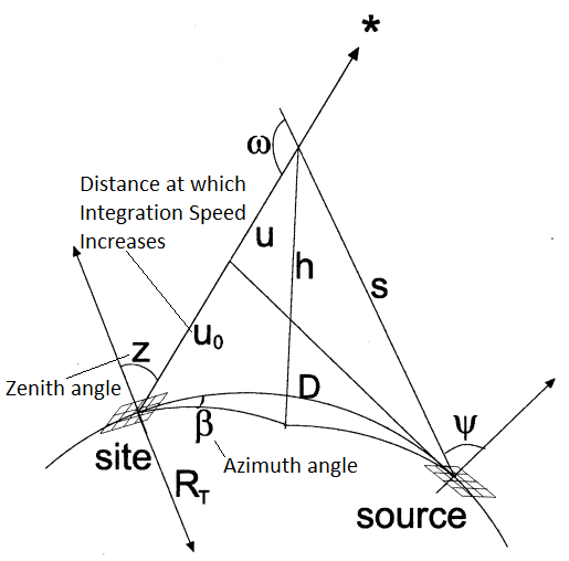
Diagram of the light propagation model created by Cinzano. Shows the relationships between the observation site and the light source. Taken and modified from REF 2, Fig. 6, p.648.

Geodesic Constants

Radius of the Earth at the equator, \(R_{equator}\), assuming an ellipsoidal surface:

Radius of the Earth at the poles, \(R_{polar}\), assuming an ellipsoidal surface:

Atmospheric Constants

\(N_{m,0}\), molecular density at sea level (Cinzano et al., 2000, p.645)

\(c_{isa}\), the inverse scale altitude of aerosols. For each kilometer above sea level, the molecular density of aerosols is assumed to be reduced by a factor of 0.104 (Cinzano et al., 2000, p.645).

For the general case, the ratio \(K\) of aerosol scattering to gas molecule scattering is assumed to be 1:1. A higher number indicates greater optical thickness, a lower number clearer skies (Falchi et al., 2016, p.10). For the western United States, a lower setting like 0.5 might be more representative of typical conditions.

\(a_{sha}\), the scale height of aerosols (Cinzano et al., 2000, p.646)

Coefficient \(\sigma_m\) of Rayleigh scattering of visual light through a vertical cross-section of the atmosphere (Cinzano et al., 2000, p.646).

References:

1. Falchi, F., P. Cinzano, D. Duriscoe, C.C.M. Kyba, C.D. Elvidge, K. Baugh, B.A. Portnov, N.A. Rybnikova and R. Furgoni, 2016. The new workd atlas of artificial night sky brightness. Sci. Adv. 2.
2. Cinzano, P., F. Falchi, C.D. Elvidge and K.E. Baugh, 2000. The artificial night sky brightness mapped from DMSP satellite Operational Linescan System measurements. Mon. Not. R. Astron. Soc. 318.
3. Garstang, R.H., 1989. Night-sky brightness at observatories and sites. Pub. Astron. Soc. Pac. 101.

Literature¶

Foundational Papers

Cinzano, P., Falchi, F., & Elvidge, C. D. (2001). The first world atlas of the artificial night sky brightness. Monthly Notices of the Royal Astronomical Society, 328(3), 689–707. Retrieved from http://mnras.oxfordjournals.org/content/328/3/689.short

Falchi, F., Cinzano, P., Duriscoe, D., Kyba, C. C. M., Elvidge, C. D., Baugh, K., Furgoni, R. (2016). The new world atlas of artificial night sky brightness. Science Advances, 2(6), e1600377. doi:10.1126/sciadv.1600377

Garstang, R. H. (1989). Night sky brightness at observatories and sites. Publications of the Astronomical Society of the Pacific, 101(637), 306. Retrieved from http://iopscience.iop.org/article/10.1086/132436/meta

Jing, X., Shao, X., Cao, C., Fu, X., & Yan, L. (2015). Comparison between the Suomi-NPP Day-Night Band and DMSP-OLS for Correlating Socio-Economic Variables at the Provincial Level in China. Remote Sensing, 8(1), 17. https://doi.org/10.3390/rs8010017

Other Methodology Papers

Cinzano, P., Falchi, F., Elvidge, C. D., & Baugh, K. E. (2000). The artificial night sky brightness mapped from DMSP satellite Operational Linescan System measurements. Monthly Notices of the Royal Astronomical Society, 318(3), 641–657. Retrieved from http://mnras.oxfordjournals.org/content/318/3/641.short

Cinzano, P., Falchi, F., & Elvidge, C. D. (2001). Naked-eye star visibility and limiting magnitude mapped from DMSP-OLS satellite data. Monthly Notices of the Royal Astronomical Society, 323(1), 34–46. Retrieved from http://mnras.oxfordjournals.org/content/323/1/34.short

Duriscoe, D. M. (2013). Measuring anthropogenic sky glow using a natural sky brightness model. Publications of the Astronomical Society of the Pacific, 125(933), 1370. Retrieved from http://iopscience.iop.org/article/10.1086/673888/meta

Cinzano, P., & Falchi, F. (2012). The propagation of light pollution in the atmosphere. Monthly Notices of the Royal Astronomical Society, 427(4), 3337–3357. https://doi.org/10.1111/j.1365-2966.2012.21884.x

Light Pollution Impact Studies

Anderson, S. (2017, July 19). NASA DEVELOP National Program Virtual Poster Session Interview [Personal interview].

Blask, D. E., Brainard, G. C., Dauchy, R. T., Hanifin, J. P., Davidson, L. K., Krause, J. A., … Zalatan, F. (2005). Melatonin-Depleted Blood from Premenopausal Women Exposed to Light at Night Stimulates Growth of Human Breast Cancer Xenografts in Nude Rats. Cancer Research, 65(23), 11174-11184. doi:10.1158/0008-5472.CAN-05-1945

Brons, J., Bullough, J., & Rea, M. (2008). Outdoor site-lighting performance: A comprehensive and quantitative framework for assessing light pollution. Lighting Research & Technology, 40(3), 201-224. doi:10.1177/1477153508094059

Chepesiuk, R. (2009). Missing the Dark: Health Effects of Light Pollution. Environmental Health Perspectives, 117(1), A20-A27. doi:10.1289/ehp.117-a20

Dauchy, R. T., Xiang, S., Mao, L., Brimer, S., Wren, M. A., Yuan, L., … Hill, S. M. (2014). Circadian and Melatonin Disruption by Exposure to Light at Night Drives Intrinsic Resistance to Tamoxifen Therapy in Breast Cancer. Cancer Research, 74(15), 4099-4110. doi:10.1158/0008-5472.can-13-3156

Dominoni, D. M., Borniger, J. C., & Nelson, R. J. (2016). Light at night, clocks and health: from humans to wild organisms. Biology Letters, 12(2), 20160015. doi:10.1098/rsbl.2016.0015

Evans Ogden, L. J. (1996). Collision Course: The Hazards of Lighted Structures and Windows to Migrating Birds (pp. 1-46, Rep.). Fatal Light Awareness Program (FLAP). Retrieved August 8, 2017, from http://digitalcommons.unl.edu/cgi/viewcontent.cgi?article=1002&context=flap

Gallaway, T., Olsen, R. N., & Mitchell, D. M. (2010). The economics of global light pollution. Ecological Economics, 69(3), 659. doi:10.1016/j.ecolecon.2009.10.003

Gaston, K. J., Bennie, J., Davies, T. W., & Hopkins, J. (2013). The ecological impacts of nighttime light pollution: a mechanistic appraisal: Nighttime light pollution. Biological Reviews, 88(4), 912-927. doi:10.1111/brv.12036

Hill, D. (1992). The Impact of Noise and Artificial Light on Waterfowl Behaviour: A Review and Synthesis of Available Literature. Retrieved August 8, 2017, from https://www.bto.org/file/335635/download?token=7TdSzNGG

Hölker, F., Wolter, C., Perkin, E. K., & Tockner, K. (2010). Light pollution as a biodiversity threat. Trends in Ecology & Evolution, 25(12), 681-682. doi:10.1016/j.tree.2010.09.007

Kempenaers, B., Borgström, P., Loës, P., Schlicht, E., & Valcu, M. (2010). Artificial Night Lighting Affects Dawn Song, Extra-Pair Siring Success, and Lay Date in Songbirds. Current Biology, 20(19), 1735-1739. doi:10.1016/j.cub.2010.08.028

Kloog, I., Haim, A., Stevens, R. G., Barchana, M., & Portnov, B. A. (2008). Light at Night Co‐distributes with Incident Breast but not Lung Cancer in the Female Population of Israel. Chronobiology International, 25(1), 65-81. doi:10.1080/07420520801921572

Kloog, I., Stevens, R. G., Haim, A., & Portnov, B. A. (2010). Nighttime light level co-distributes with breast cancer incidence worldwide. Cancer Causes & Control, 21(12), 2059-2068. doi:10.1007/s10552-010-9624-4

Kyba, C. C., Ruhtz, T., Fischer, J., & Hölker, F. (2012). Red is the new black: how the colour of urban skyglow varies with cloud cover. Monthly Notices of the Royal Astronomical Society, 425(1), 701-708. doi:10.1111/j.1365-2966.2012.21559.x

Lacoeuilhe, A., Machon, N., Julien, J., Bocq, A. L., & Kerbiriou, C. (2014). The Influence of Low Intensities of Light Pollution on Bat Communities in a Semi-Natural Context. PLoS ONE, 9(10), e103042. doi:10.1371/journal.pone.0103042

Longcore, T., & Rich, C. (2004). Ecological light pollution. Frontiers in Ecology and the Environment, 2(4), 191-198. doi:10.2307/3868314

McFadden, E., Jones, M. E., Schoemaker, M. J., Ashworth, A., & Swerdlow, A. J. (2014). The Relationship Between Obesity and Exposure to Light at Night: Cross-Sectional Analyses of Over 100,000 Women in the Breakthrough Generations Study. American Journal of Epidemiology, 180(3), 245-250. doi:10.1093/aje/kwu117

Moran, M., & Salisbury, D. F. (2006, August 21). Constant lighting may disrupt development of preemie’s biological clocks. Retrieved August 08, 2017, from https://news.vanderbilt.edu/2006/08/21/constant-lighting-may-disrupt-development-of-preemies-biological-clocks-58939/

Navigant Consulting, Inc. (2012, January). US Department of Energy (United States, Department of Energy, Office of Energy Efficiency & Renewable Energy). Retrieved June 21, 2017, from https://www1.eere.energy.gov/buildings/publications/pdfs/ssl/2010-lmc-final-jan-2012.pdf

Ohta, H., Mitchell, A. C., & McMahon, D. G. (2006). Constant Light Disrupts the Developing Mouse Biological Clock. Pediatric Research, 60(3), 304-308. doi:10.1203/01.pdr.0000233114.18403.66

Pennsylvania Outdoor Lighting Council. (2015, October 21). Electricity Cost of Waste Outdoor Lighting, United States - 2014 [Chart]. In Pennsylvania Outdoor Lighting Council. Retrieved June 21, 2017, from http://www.polcouncil.org/polc2/US_Annual_Electricity_Cost_Waste_Outdoor_Lighting_2014.pdf

Rand, A. S., Bridarolli, M. E., Dries, L., & Ryan, M. J. (1997). Light Levels Influence Female Choice in Túngara Frogs: Predation Risk Assessment? Copeia, 1997(2), 447-450. doi:10.2307/1447770

Ruggles, C. L., & Cotte, M. (2010). Heritage Sites of Astronomy and Archaeoastronomy in the context of the UNESCO World Heritage Convention: A Thematic Study. Retrieved July 13, 2017, from http://www.astronomicalheritage.org/index.php?option=com_content&view=article&id=28&Itemid=33

Salmon, M., Tolbert, M. G., Painter, D. P., Goff, M., & Reiners, R. (1995). Behavior of Loggerhead Sea Turtles on an Urban Beach. II. Hatchling Orientation. Journal of Herpetology, 29(4), 568-576. doi:10.2307/1564740

Schernhammer, E. S., Laden, F., Speizer, F. E., Willett, W. C., Hunter, D. J., Kawachi, I., & Colditz, G. A. (2001). Rotating night shifts and risk of colorectal cancer in women participating in the nurses health study. Journal of the National Cancer Institute, 93(20), 1563-1568. Retrieved from https://blog.lsgc.com/wp-content/uploads/2016/04/08.-Schernhammer-2001-Nurses-Health-Study.pdf

Solano Lamphar, H. A., & Kocifaj, M. (2013). Light Pollution in Ultraviolet and Visible Spectrum: Effect on Different Visual Perceptions. PLoS ONE, 8(2), e56563. doi:10.1371/journal.pone.0056563

Squires, W. A., & Hanson, H. E. (1918). The Destruction of Birds at the Lighthouses on the Coast of California. The Condor, 20(1), 6-10. doi:10.2307/1362354

Vinogradova, I. A., Anisimov, V. N., Bukalev, A. V., Semenchenko, A. V., & Zabezhinski, M. A. (2009). Circadian disruption induced by light-at-night accelerates aging and promotes tumorigenesis in rats. Aging, 1(10), 855-865. doi:10.18632/aging.100092

Wyoming Stargazing. (2017). Save Our Night Skies. Retrieved June 21, 2017, from http://www.wyomingstargazing.org/save-our-night-skies/